Node Shapes in Two-Dimensions¶

In the previous sections, we focused on one-dimensional problems. This tutorial expands the scope to two-dimensional problems, highlighting the differences and challenges involved. As the number of dimensions increases, managing nodes becomes progressively more complex. While in 1D a node is simply a point, such as a zero-crossing, in 2D, nodes can take on various shapes. These distinctions are explained in detail below.

Define the System to Solve¶

The interface to SigSpace is designed to handle problems across different dimensions efficiently, requiring only minor modifications to previously introduced examples. If you haven’t gone through the earlier tutorials, particularly the one on quantum wells, it’s recommended to review them first to understand the basic commands and concepts.

The first step is to define the system we want to study. Similar to the 1D case, the system is described using the Hamiltonian. The primary change for 2D problems is that the Hamiltonian now incorporates two dimensions during its creation. This is done by the sdims parameter in sg.Hamiltonian(sdims=2):

In addition to updating the Hamiltonian, the potential callback function also requires modification. The argument pts is now a two-dimensional array representing the grid points, with a shape of (number of points, 2).

The function call np.all(np.abs(pts) < 4, axis=1) evaluates whether each point lies within a square box of side length 8, centered at the origin. This condition is used to define the potential. Multiplying the result by -1 makes the potential attractive, as we aim to establish a bound state.

The command sg.quickplot(sol) then automatically generates a mesh plot, visualizing the wave function confined within the rectangular box.

Nodes Shapes in Two-Dimensions¶

From 1D to 2D Nodes¶

In the 1D case (refer to the tutorial on 1D excited states), nodes are added using solver.nodes.add(). Since nodes in 1D are simple points, it is sufficient to specify the number of nodes, and the solver determines their positions automatically.

In 2D, however, the situation is more complex. Nodes are no longer just points; they can have various shapes, requiring both their location and geometry to be explicitly defined.

Planar Nodes¶

The simplest node shape in 2D is a straight line dividing the positive and negative regions of the wave function. These are referred to as planar nodes in SigSpace.

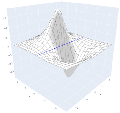
In the figure below, an excited state with a planar node is depicted. The node is represented by a blue line:

A planar node is described using the PlanarNode object. Its constructor requires two arguments: a point on the node and its normal vector (i.e., the direction perpendicular to the node). For example:

node = sg.PlanarNode(point=[0, 0], normal=[1, 0])

It’s important to note that the solver is highly sensitive to the exact placement of nodes. If a node is not positioned precisely, the solver may fail to converge.

Current Limitations and Future Development¶

Currently, SigSpace supports only a single planar node. Future releases will extend support to additional node shapes and the combination of multiple nodes. This limitation means it may not always be possible to calculate the next excited state if its corresponding node has a different shape.

Estimating Nodes for Excited States¶

To calculate an excited state, SigSpace can estimate the location of nodes based on the ground state solution. These estimated nodes can be accessed from a solution object as follows:

The code snippet displays a list of planar nodes suitable for the given problem. Each node is characterized by two parameters: p, a point lying on the node, and n, the direction (or normal vector) of the node.

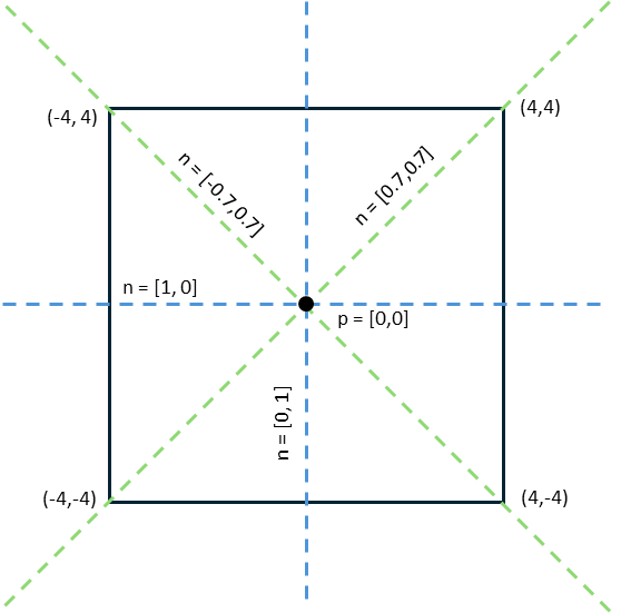
For the quadratic potential used in this example, the locations of the nodes are visualized in the image below:

Due to the symmetry of the potential, two nodes are oriented perpendicular to the boundary of the potential (depicted as dashed blue lines), while the other two nodes align along the diagonals of the box potential (shown as dashed green lines). This symmetry allows for four different excited states, each associated with a single planar node.

The detected nodes can then be passed to the solver to calculate the corresponding excited state.

The command solver.nodes.add(node) specifies which node should be included in the solution.

By visualizing the result with quickplot, we can observe the positive and negative regions of the wave function:

State Degeneracy¶

As expected, the energy of the excited state is slightly higher than the ground state. However, the energy differences between the excited states are very small. Notably, the diagonal (green) and perpendicular (blue) nodes yield the same energy, as the corresponding wave functions are identical, differing only by a 90° rotation.

This raises the question: are all these solutions truly degenerate energy levels? Degenerate states are characterized by having the same energy but distinct (linearly independent) wave functions.

Given the current level of accuracy, it is unclear whether the states genuinely share the exact same energy. To improve the results and achieve greater precision, several modifications can be made to the code:

1. Increase Grid Resolution Use solver.grid((-10, 10, 50)) to increase the number of grid points. A finer grid provides more accurate wave functions and energy values.

2. Adjust Damping Factor α The damping factor controls the step size during iterations. By default, it is set automatically by the solver. If convergence issues arise, manually reducing solver.alpha can improve results. This is particularly important when increasing grid resolution, as a smaller alpha value may be necessary. However, note that reducing alpha will increase computation time.

3. Refine the Stopping Criterion (stop_error) The stopping criterion determines when the calculation will halt based on energy accuracy. The default value is 1e-2. Decreasing it to 1e-3 or lower can further reduce the error.

4. Limit Maximum Iterations (max_iterations) By default, the solver allows infinite iterations. When reducing stop_error, it is advisable to set a limit on max_iterations. This ensures the solver stops even if the desired accuracy is unattainable.

5. Enable Intermediate Updates (print_iter) For long-running calculations, use solver.print_iter = 1000 to receive updates every 1000 iterations. This provides intermediate progress without needing to wait for the calculation to finish.

With these modifications applied, we can rerun the calculation to obtain more accurate results.

The resulting energies are now much closer to each other. However, even with further increases in accuracy, a small difference between the energies of the nodes remains. This indicates that full degeneracy of the energy levels does not occur. The small differences arise because the wave functions, while similar, are not completely identical.

Rotationally Symmetric Problems¶

Degenerate energy levels are typically associated with wave functions that are linearly independent. Such degeneracy often occurs in rotationally symmetric problems. Due to the symmetry, a planar node can align in any direction, leading to multiple equivalent solutions.

The following example demonstrates this behavior:

In SigSpace, the location of the node (in this case, at [0, 0]) is estimated automatically. However, the direction of the node is not fixed and must be specified manually to solve the problem. This can be done using the set_normal method: